Chapter 4 Analysis of Economic Variables

Exogenous shocks are unpredictable events affecting a system of variables. For example, a monetary policy shock affects a country’s output and inflation.

ARMA models are useful to analyse the response of economic variables to these shocks.

estimate the expected response of these variables, modelled with ARMA processes, to a shock.

4.1 Impulse Response Function

The Impulse Response Function, \(\widetilde{y}_{t}\), describes the expected response of a variable to an exogenous shock, which occurs at time \(t=s\). The shock could be of magnitude 1 or one standard deviation.

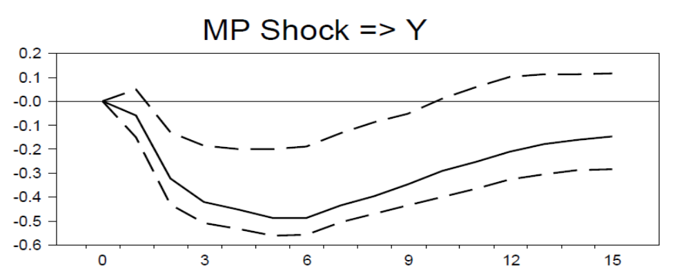
Figure 4.1: Impulse/shock: Fed Funds interest rate, Response: GDP

A 1% shock in the interest rate/monetary policy decreases GDP for the first 6 months. After 6 months, GDP starts increasing again.

The value of the variable before the shock happens is a fixed value \(y\).

The IRFs are given by the following set of equations: \[\begin{align} \widetilde{y}_t&=y \;\;\;\;\; \forall t<s \\ \widetilde{y}_t&=y+\frac{\partial y_t}{\partial \epsilon_s}\cdot 1 \;\;\;\;\; \forall t\geq s \tag{4.1} \end{align}\]

Focus the response of the time series \(y\) to this exogenous shock.

Assume the time series is modelled as an AR(1) \[\begin{align*} y_t&=\phi y_{t-1}+\epsilon_t \end{align*}\] At time \(t\) there is a shock of magnitude 1.

We estimate the expected behaviour of \(y\) in the next three periods using the Impulse Response Function.

At time \(t+1\), the next period, the AR(1) is given by: \[\begin{align} y_{t+1}&=\phi_1 y_{t}+\epsilon_{t+1} \end{align}\] Substitute \(y_t\): \[\begin{align} y_{t+1}&=\phi (\phi y_{t-1}+\epsilon_t)+\epsilon_{t+1}=\phi^2 y_{t-1}+\phi\epsilon_t+\epsilon_{t+1} \end{align}\]

Then, the effect of the shock on the time series is the partial derivative of \(y_t\) with respect to \(\epsilon_t\): \[\begin{align} \frac{\partial y_{t+1}}{\partial\epsilon_t}&=\phi \end{align}\] So, the response of \(y_t\) one period after the shock occurred is \[\begin{align} \widetilde{y}_{t+1}&=y+\frac{\partial y_{t+1}}{\partial \epsilon_t}\cdot 1= y+\phi \cdot 1 \end{align}\]

Repeat the process for two and three periods after the shock.
After two periods, \(t+2\), \[\begin{align} y_{t+2}&=\phi^3 y_{t-1}+\phi^2\epsilon_t+\phi\epsilon_{t+1} +\epsilon_{t+2} \frac{\partial y_{t+2}}{\partial\epsilon_t}&=\phi^2 \end{align}\] Then, the IRF after two periods is \[\begin{align} \widetilde{y}_{t+2}&=y+\phi^2 \cdot 1 \end{align}\] Similarly for the IRF after three steps ahead: \(\widetilde{y}_{t+3}=y+\phi^3 \cdot 1\).

Alternatively, use the Wold representation theorem (see ): \[\begin{align} y_t&=\phi y_{t-1}+\epsilon_t \rightarrow y_t=\sum_{j=0}^{\infty}\psi_j\epsilon_{t-j} \end{align}\] where we use the substitution \(\psi_j=\phi^j\).
Then, we get: \[\begin{align} \frac{\partial y_{t}}{\partial\epsilon_s}&=\psi_{t-s}=\phi^{t-s} \end{align}\] The IRFs at 1,2, and 3 steps ahead are given by: \[\begin{align} \tilde{y}_{t+1}&=y+\frac{\partial y_{t+1}}{\partial\epsilon_s}\cdot 1= y+\psi_1=y+\phi \tilde{y}_{t+2}&=y+\frac{\partial y_{t+2}}{\partial\epsilon_s}\cdot 1= y+\psi_2=y+\phi^2 \tilde{y}_{t+3}&=y+\frac{\partial y_{t+3}}{\partial\epsilon_s}\cdot 1= y+\psi_3=y+\phi^3 \end{align}\]

Notice two aspects.

models compute IRFs, including multiple variables and addressing the misspecification issue.

4.2 Local Projections

The Local Projection (LP) methods are useful to compute IRFs addressing possible misspecification in the model and considering multiple variables.

This method estimates a regression for each variable and for each step ahead \(s\).

The LP specification for \(y_t\) at step ahead \(s\) is: \[\begin{align} y_{t+s}&=\beta_s x_t+\sum_{j=1}^l \gamma_{s,l}^{\prime}y_{t-l}+\sum_{j=1}^l\delta_{s,l}^{\prime}x_{t-l}+\epsilon_{t+s} \tag{4.2} \end{align}\] \(y_{t+s}\) includes both the lags of \(y_t\) and of \(x_t\) (second and term terms on the RHS).

Let \(y_t\) be real GDP of country \(C\) and \(x_t\) real interest rate.
Assume the interest rate increases suddenly.
Our goal is to estimate the effect of this increase on GDP in the next quarters/years.
At time \(t+1\), estimate the regression in eq. (4.2) with 1 lag using OLS: \[\begin{align} y_{t+1}&=\beta_1 x_t+ \gamma_{1,1}y_{t-1}+\delta_{1,1}x_{t-1}+\epsilon_{t+1} \end{align}\] Repeat for estimating the effect at time \(t+2\): \[\begin{align} y_{t+2}&=\beta_2 x_t+ \gamma_{2,1}y_{t-1}+\delta_{2,1}x_{t-1}+\epsilon_{t+1} \end{align}\] And so on. In the end, the coefficients \(\beta_1\), \(\beta_2\) estimate the effect of an increase today in interest rate on GDP over the future periods.

Focus the estimated \(\beta_s\).
\(\beta_s\) represents the impact of the shock on the variable \(y_t\) - so it is the Local Projection impulse response.

Estimate the equations for both time series and for each step ahead \(s=1,2,3,\ldots\) using OLS.

For each horizon \(s\), the LP impulse response, \(\beta_s\), is given by the difference between the expected value of \(y_{t+s}\) if the shock has occurred and if it has not: \[\begin{equation} \beta_s=\mathbb{E}(y_{t+s} |x_t=1,y_t,x_t) - \mathbb{E}(y_{t+s} |x_t =0,y_t,x_t) \end{equation}\] Note when estimating, include heteroskedasticity- and autocorrelation-consistent (HAC) standard errors.