Introduction to Time Series
2026-03-21
1 Introduction
“Econometrics is the science and art of using economic theory and statistical techniques to analyze economic data.’’ (Stock, J.H., Watson, M.W., 2018)
1.1 Types of data
Cross section: data on different entities (workers, consumers, firms, etc.) collected at a single time period (e.g. number of inhabitants per postcode in 2010).

Figure 1.1: Cross section: time variable year 2010, ID variable postcode

Figure 1.2: Time series: time variable date, ID variable Netherlands Source: FRED Real GDP Netherlands
Panel data: data for multiple entities in which each entry is observed at two or more time periods (e.g. number of inhabitants in postcodes over time).

Figure 1.3: Panel data: time variable year, ID variable postcode

Figure 1.4: Example of a time series: \(CO_2\) emissions
1.2 Time Series
A time series or a time-varying process is a set of observations \(\{y_t\}\) on a variable over a time period.
\[\begin{align}
y_1,\ldots,& y_n \implies \{y_t\} \;\;\;\;\;\ t=1,\ldots,n
\end{align}\]
The is the value of \(y\) at time \(t\), .
The (or lagged value) is the value of \(y_t\) in the previous period, .
The of \(y\) is its value \(p\) periods before \(t\), .
The difference between the value of \(y\) at time \(t\) and \(t-1\) is called
\[\begin{align}
\Delta y_t&= y_t-y_{t-1}
\end{align}\]
where \(\Delta\) is the difference operator.
1.2.1 Time Series properties
Stationary data: time-series data that has a constant mean value over time.
This condition is very helpful for predicting and forecasting the time series, hence it is a relevant condition.
In details, the stationarity condition implies that the mean, variance and covariance of the time series \(y_t\) should be constant over time and finite: \[\begin{align} \mathbb{E}(y_t)&=\mu \;\;\;\;\;\;\;\; \forall t \text{$\mathbb{V}$ar}(y_t)&=\gamma(0) \;\;\;\; \forall t \text{$\mathbb{C}$ov}(y_{t+h},y_t)&=\gamma(h)\;\;\;\; \forall t \end{align}\]
Expected value: the mean of the series \(y_t\) is the long-run average.Variance: the dispersion or spread of a probability distribution. It is the expected value of the square of the deviation of the variable from its expected value.
Autocovariance: the covariance between two values of the time series at different points in time.
2 Time Series Processes
The time series models we discuss are:
White noise (WN) Moving Average (MA) Autoregressive (AR) Random Walk (RW)Autoregressive Moving Average (ARMA)
2.1 White Noise
White noise (WN) process: \(\epsilon_t\) is a time series with the following characteristics \[\begin{align} \mathbb{E}(\epsilon_t)&=0 \text{$\mathbb{V}$ar}(\epsilon_t)&=\mathbb{E}(\epsilon_t^2)=\sigma^2 < \infty \text{$\mathbb{C}$ov}(\epsilon_t, \epsilon_{t-k})&=\gamma(k) =0 \;\;\;\;\;\;\;\; \text{for k}>0 \end{align}\]
The autocovariance \(\gamma(k)\) of a white noise is 0. This indicates that the time series does not have memory of itself. So, there is no persistence in the white noise: \(\epsilon_t\) is not similar or influenced by \(\epsilon_{t-k}\).
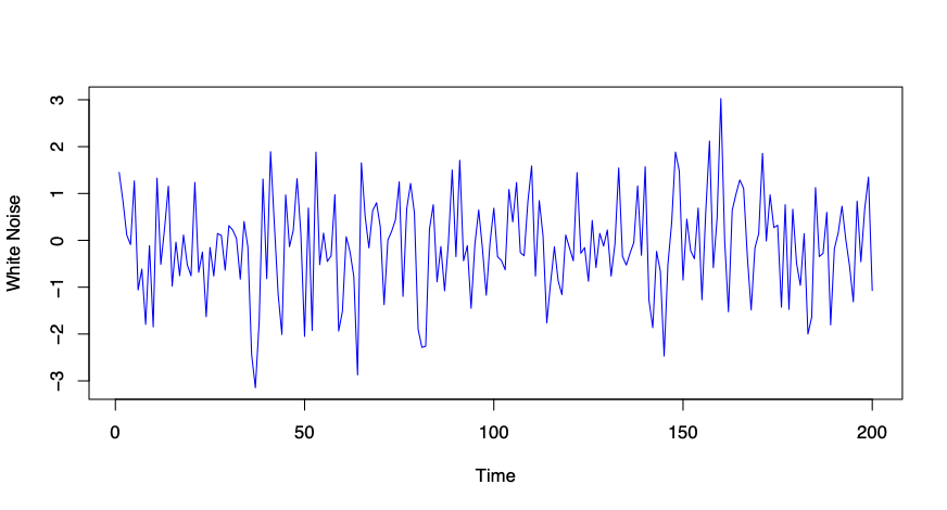
Figure 2.1: White noise - Example
2.2 Moving Average
Moving Average (MA) process: the time series \(y_t\) depends on the current and the past values of the error term \(\epsilon_t\).
Consider that \(y_t\) depends on the first lag of \(\epsilon_t\), \(\epsilon_{t-1}\).
Then, the time series follows a moving average process of order 1, denoted MA(1):
\[\begin{equation*}
y_t=\mu+\epsilon_t+\theta \epsilon_{t-1}, \;\;\;\;\;\; \epsilon_t\sim \mathcal{N}(0,\sigma^2)
\end{equation*}\]
where \(\mu\) is an constant, \(\sigma^2\) is the variance of \(\epsilon_t\).
Consider that \(y_t\) depends on the \(q\) lags of \(\epsilon_t\). Then, the moving average process is of order \(q\), MA(q). \[\begin{equation*} y_t=\mu+\epsilon_t+\theta \epsilon_{t-1}+\ldots+\theta_q \epsilon_{t-q} \end{equation*}\]
Stationarity condition holds.\[\gamma(1) = \text{$\mathbb{C}$ov}(\mu+\epsilon_t+\theta \epsilon_{t-1}, y_{t-1})\]
Note: \(y_{t-1} = \mu + \epsilon_{t-1}+ \theta \epsilon_{t-2}\). Assume that the error terms are serially independent, i.e.~\(\epsilon_t \perp \epsilon_{t-k} \;\; \forall k\geq1\).
\[\begin{align*} \text{$\mathbb{C}$ov}(\mu&+\epsilon_t+\theta \epsilon_{t-1}, y_{t-1}) = \text{$\mathbb{C}$ov}(\mu, y_{t-1})+&\text{$\mathbb{C}$ov}(\epsilon, y_{t-1})+ \text{$\mathbb{C}$ov}(\theta\epsilon_{t-1}, y_{t-1}) \end{align*}\]
\[\text{$\mathbb{C}$ov}(y_t, y_{t-1})=\gamma(1)=\theta\text{$\mathbb{V}$ar}(\epsilon_{t-1})= \theta \sigma^2\] \[\text{$\mathbb{C}$ov}(y_t, y_{t-k})=\gamma(k)=0 \;\;\;\; \text{for} \;\; k>1\]
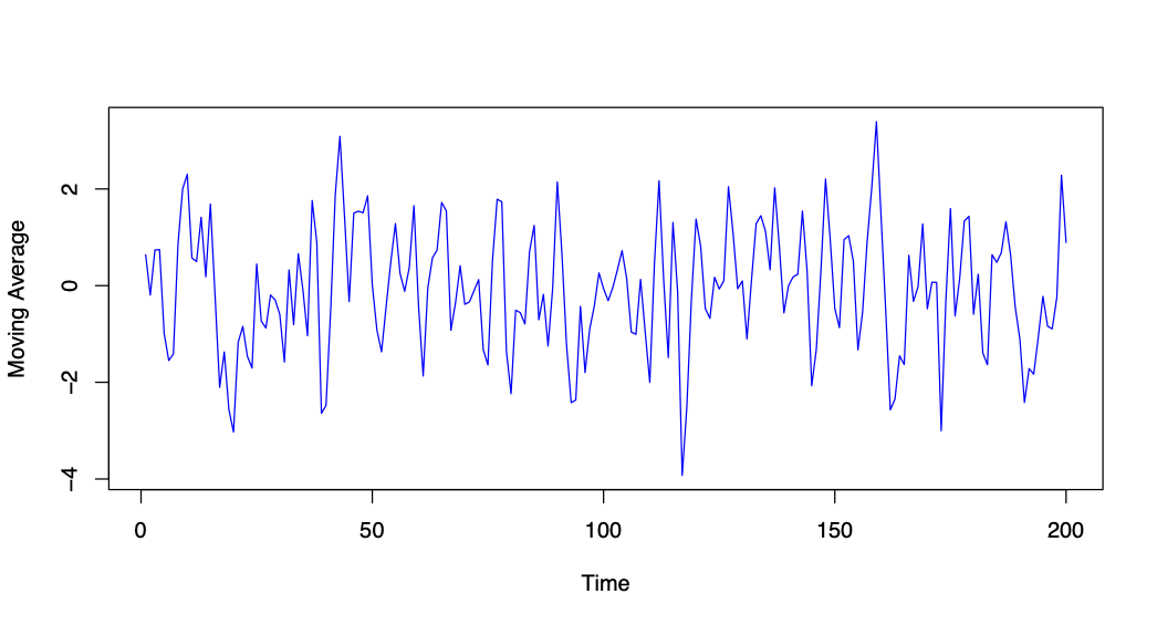
Figure 2.2: The coefficient \(\theta\) is set to 0.7
2.3 Autoregressive process
Autoregressive (AR) process: the time series \(y_t\) depends on its previous values and on an error term \(\epsilon_t\).
Consider that \(y_t\) depends only on its first lag and on \(\epsilon_t\). Then, the time series follows an autoregressive process of order 1, denoted AR(1): \[\begin{equation*} y_t=\mu+\phi y_{t-1}+\epsilon_t, \;\;\;\;\;\; \epsilon_t\sim \mathcal{N}(0,\sigma^2) \end{equation*}\] where \(\mu\) is an intercept, \(\sigma^2\) is the variance of \(\epsilon_t\).
Consider that \(y_t\) depends on its \(p\) past values. Then, the autoregressive process is of order \(p\), AR(p).
\[y_t=\mu+\phi y_{t-1}+\ldots+\phi_p y_{t-p}+\epsilon_t\]
The stationarity condition holds if \(|\phi|\) is lower than 1.
Let’s consider an AR(1) process. Its statistical properties are:
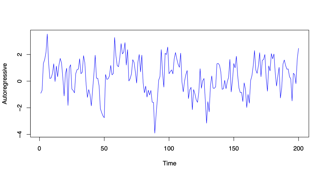
Figure 2.3: The coefficient \(\phi\) is set to 0.7
2.4 Wold Representation Theorem
A (covariance) stationary time series \(y_t\) can be represented as a Moving Average process of order infinity, MA(\(\infty\)): \[\begin{align*} y_t&=\sum_{j=0}^\infty\psi_j\epsilon_{t-j} \end{align*}\] To see how, consider an AR(1) process: \[\begin{align*}\label{ar1} y_t&=\phi y_{t-1}+\epsilon_t \end{align*}\] Substitute \(y_{t-1}\): \[\begin{align*} y_t&=\phi^2 y_{t-2}+ \phi \epsilon_{t-1} +\epsilon_t \end{align*}\] Recursively substitute \(y_{t-2}\) to \(y_{t-j}\), until you get: \[\begin{align*} y_t&=\phi^j \epsilon_{t-j}+ \ldots + \phi \epsilon_{t-1} +\epsilon_t= \sum_{j=0}^\infty \psi_j \epsilon_{t-j} \end{align*}\] where \(\psi_j =\phi^j\) and \(\sum_{j=0}^\infty|\psi_j|<\infty\).
2.5 Autoregressive Moving Average Process
Autoregressive Moving Average (ARMA) process: the time series \(y_t\) is formed by an autoregressive component and a moving average one.
The representation of ARMA(1,1) combines AR(1) and MA(1): \[ y_t=\phi y_{t-1}+\epsilon_t+\theta \epsilon_{t-1}\]
The ARMA process of order (p,q) is:
\[y_t=\phi_1 y_{t-1}+\ldots+\phi_p y_{t-p}+\epsilon_t+\theta_1 \epsilon_{t-1}+\ldots+\theta_q \epsilon_{t-q}\]
The stationarity condition holds if \(|\phi|\) is lower than 1.
Notice that ARMA(1,0) is an AR(1) and ARMA(0,1) is an MA(1).
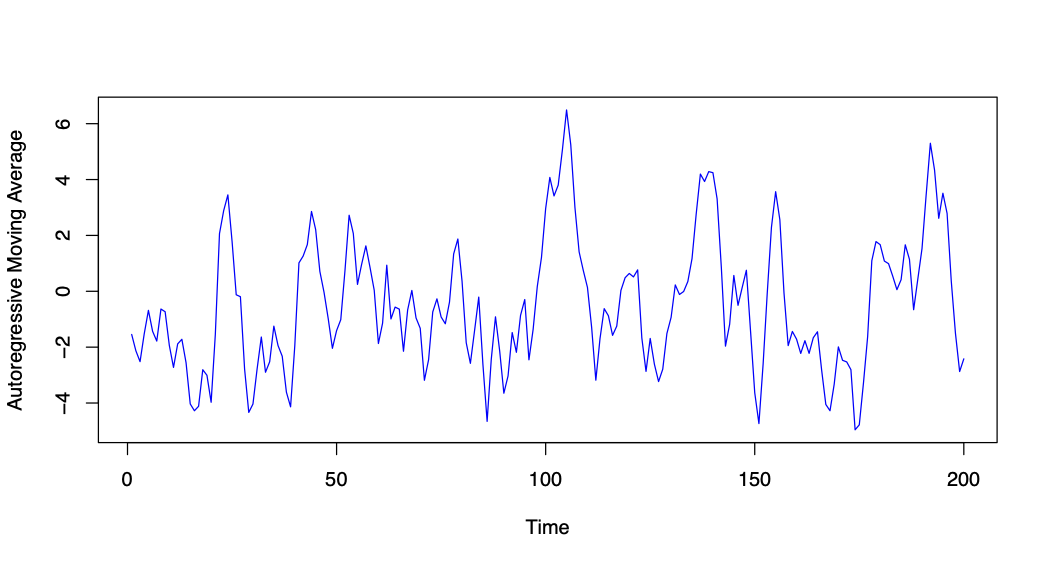
Figure 2.4: The coefficient \(\phi\) and \(\theta\) are both set to 0.7
2.6 Random Walk
If the parameter \(\phi=1\), the process is a random walk (RW): \[\begin{align*} y_t&=y_{t-1}+\epsilon_t \end{align*}\]
This time series is a sum of random shocks \(\epsilon_t\) with \(t\) from time 1 until \(t\).Repeat steps and for all \(t\) until you get: \[y_t=\epsilon_1+\ldots+\epsilon_t\]
The stationarity condition **doesn’t hold.
Note that \(\epsilon_t \; \forall t\) is a white noise process, \(\epsilon_t \sim \mathcal{N}(0, \sigma^2)\).
The variance increases with \(t\) \(\implies\) the variance depends on time \(\implies\) non-stationary process.
The variance increases with \(t\) \(\implies\) the variance depends on time \(\implies\) non-stationary process.
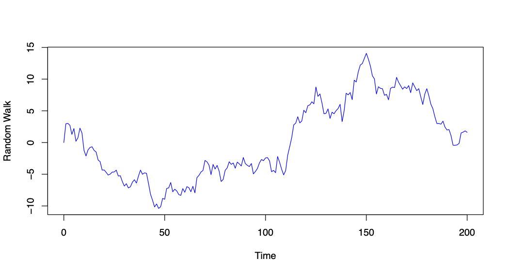
Figure 2.5: Random Walk - Example
3 How to deal with a non-stationary process?
The RW is a simple nonstationary process. 1
The accumulation of random shocks, \(\epsilon_t\), creates a stochastic trend.
This causes the non-stationarity.
To solve this problem, a solution is to take the first difference: \(\Delta y_t=y_t - y_{t-1}\).
The first difference of a random walk process would be the white noise:
\[\begin{align*}
\Delta y_t&=y_t - y_{t-1}=\epsilon_t
\end{align*}\]
Assume the data follow an AR(1) process: \[\begin{align*} y_t&=\phi y_{t-1}+\epsilon_t \end{align*}\] Focus the coefficient \(\phi\). Is it equal to 1 (unit root) or smaller than 1?
We can use the Dickey-Fuller (DF) test to check for stationarity and answer this question.
3.1 Dickey-Fuller test
The Dickey-Fuller test tests the null hypothesis of \(\phi\) being equal to 1, against the alternative hypothesis of \(\phi\) being lower than 1. Using a compact notation, DF testsThe DF test is similar to the \(t\)-test
\[\begin{align*}
DF&=\frac{\hat{\phi}-1}{SE(\hat{\phi})}
\end{align*}\]
where \(\hat{\phi}\) is the parameter \(\phi\) of AR(1) estimated using OLS.
The \(t\)-test follows a Student t-distribution, while the DF test follows a .
4 Analysis of Economic Variables
Exogenous shocks are unpredictable events affecting a system of variables. For example, a monetary policy shock affects a country’s output and inflation.
ARMA models are useful to analyse the response of economic variables to these shocks.
estimate the expected response of these variables, modelled with ARMA processes, to a shock.
4.1 Impulse Response Function
The Impulse Response Function, \(\widetilde{y}_{t}\), describes the expected response of a variable to an exogenous shock, which occurs at time \(t=s\). The shock could be of magnitude 1 or one standard deviation.
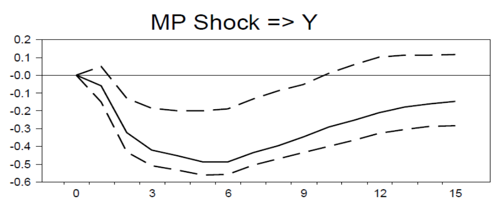
Figure 4.1: Impulse/shock: Fed Funds interest rate, Response: GDP
A 1% shock in the interest rate/monetary policy decreases GDP for the first 6 months. After 6 months, GDP starts increasing again.
The value of the variable before the shock happens is a fixed value \(y\).
The IRFs are given by the following set of equations: \[\begin{align} \widetilde{y}_t&=y \;\;\;\;\; \forall t<s \\ \widetilde{y}_t&=y+\frac{\partial y_t}{\partial \epsilon_s}\cdot 1 \;\;\;\;\; \forall t\geq s \tag{4.1} \end{align}\]
Focus the response of the time series \(y\) to this exogenous shock.
Assume the time series is modelled as an AR(1) \[\begin{align*} y_t&=\phi y_{t-1}+\epsilon_t \end{align*}\] At time \(t\) there is a shock of magnitude 1.
We estimate the expected behaviour of \(y\) in the next three periods using the Impulse Response Function.
At time \(t+1\), the next period, the AR(1) is given by: \[\begin{align} y_{t+1}&=\phi_1 y_{t}+\epsilon_{t+1} \end{align}\] Substitute \(y_t\): \[\begin{align} y_{t+1}&=\phi (\phi y_{t-1}+\epsilon_t)+\epsilon_{t+1}=\phi^2 y_{t-1}+\phi\epsilon_t+\epsilon_{t+1} \end{align}\]
Then, the effect of the shock on the time series is the partial derivative of \(y_t\) with respect to \(\epsilon_t\): \[\begin{align} \frac{\partial y_{t+1}}{\partial\epsilon_t}&=\phi \end{align}\] So, the response of \(y_t\) one period after the shock occurred is \[\begin{align} \widetilde{y}_{t+1}&=y+\frac{\partial y_{t+1}}{\partial \epsilon_t}\cdot 1= y+\phi \cdot 1 \end{align}\]
Repeat the process for two and three periods after the shock.
After two periods, \(t+2\),
\[\begin{align}
y_{t+2}&=\phi^3 y_{t-1}+\phi^2\epsilon_t+\phi\epsilon_{t+1} +\epsilon_{t+2}
\frac{\partial y_{t+2}}{\partial\epsilon_t}&=\phi^2
\end{align}\]
Then, the IRF after two periods is
\[\begin{align}
\widetilde{y}_{t+2}&=y+\phi^2 \cdot 1
\end{align}\]
Similarly for the IRF after three steps ahead: \(\widetilde{y}_{t+3}=y+\phi^3 \cdot 1\).
Alternatively, use the Wold representation theorem (see ):
\[\begin{align}
y_t&=\phi y_{t-1}+\epsilon_t \rightarrow y_t=\sum_{j=0}^{\infty}\psi_j\epsilon_{t-j}
\end{align}\]
where we use the substitution \(\psi_j=\phi^j\).
Then, we get:
\[\begin{align}
\frac{\partial y_{t}}{\partial\epsilon_s}&=\psi_{t-s}=\phi^{t-s}
\end{align}\]
The IRFs at 1,2, and 3 steps ahead are given by:
\[\begin{align}
\tilde{y}_{t+1}&=y+\frac{\partial y_{t+1}}{\partial\epsilon_s}\cdot 1= y+\psi_1=y+\phi
\tilde{y}_{t+2}&=y+\frac{\partial y_{t+2}}{\partial\epsilon_s}\cdot 1= y+\psi_2=y+\phi^2
\tilde{y}_{t+3}&=y+\frac{\partial y_{t+3}}{\partial\epsilon_s}\cdot 1= y+\psi_3=y+\phi^3
\end{align}\]
models compute IRFs, including multiple variables and addressing the misspecification issue.
4.2 Local Projections
The Local Projection (LP) methods are useful to compute IRFs addressing possible misspecification in the model and considering multiple variables.
This method estimates a regression for each variable and for each step ahead \(s\).The LP specification for \(y_t\) at step ahead \(s\) is: \[\begin{align} y_{t+s}&=\beta_s x_t+\sum_{j=1}^l \gamma_{s,l}^{\prime}y_{t-l}+\sum_{j=1}^l\delta_{s,l}^{\prime}x_{t-l}+\epsilon_{t+s} \tag{4.2} \end{align}\] \(y_{t+s}\) includes both the lags of \(y_t\) and of \(x_t\) (second and term terms on the RHS).
Let \(y_t\) be real GDP of country \(C\) and \(x_t\) real interest rate.
Assume the interest rate increases suddenly.
Our goal is to estimate the effect of this increase on GDP in the next quarters/years.
At time \(t+1\), estimate the regression in eq. (4.2) with 1 lag using OLS:
\[\begin{align}
y_{t+1}&=\beta_1 x_t+ \gamma_{1,1}y_{t-1}+\delta_{1,1}x_{t-1}+\epsilon_{t+1}
\end{align}\]
Repeat for estimating the effect at time \(t+2\):
\[\begin{align}
y_{t+2}&=\beta_2 x_t+ \gamma_{2,1}y_{t-1}+\delta_{2,1}x_{t-1}+\epsilon_{t+1}
\end{align}\]
And so on. In the end, the coefficients \(\beta_1\), \(\beta_2\) estimate the effect of an increase today in interest rate on GDP over the future periods.
Focus the estimated \(\beta_s\).
\(\beta_s\) represents the impact of the shock on the variable \(y_t\) - so it is the Local Projection impulse response.
Estimate the equations for both time series and for each step ahead \(s=1,2,3,\ldots\) using OLS.
For each horizon \(s\), the LP impulse response, \(\beta_s\), is given by the difference between the expected value of \(y_{t+s}\) if the shock has occurred and if it has not: \[\begin{equation} \beta_s=\mathbb{E}(y_{t+s} |x_t=1,y_t,x_t) - \mathbb{E}(y_{t+s} |x_t =0,y_t,x_t) \end{equation}\] Note when estimating, include heteroskedasticity- and autocorrelation-consistent (HAC) standard errors.
Non-stationary process: time-series data with mean value that can either rise or fall over time.↩︎